III. What came first, the chicken or the egg? Toxoplasmosis, or a change in behavior?
From the beginning, I encountered the following problem: if there were differences in the psychological profiles of Toxo positive versus negative persons, then it wouldn’t be clear whether Toxoplasma had caused the differences, or whether particular psychological traits made one more likely to be infected. And it’s hard to decide between these two possibilities. Of course, if we were studying animals other than humans, then the solution would be quite simple. We could separate the animals into two identical groups – a control and an experimental group – and infect that latter with the parasite (see Box 15 Popular mistakes when making a control group).
Box 15 Popular mistakes when making a control groupWhen preparing experimental studies, we should always try to correctly set-up the control group. Before the experiment begins, the individuals in the control group cannot be different in any way from those in the experimental group – the ones we expose to the studied factor, such as Toxoplasma infection. Otherwise, any differences we observe between the infected and uninfected animals might not be due to the parasite, but stem from differences that existed before the experiment. A good way to mess up your experiments is by setting up two cages, one for the infected and the other for the uninfected animals. Then we take twenty mice out of their crate, one by one, and set them in the control group cage; we repeat the process for the experimental cage. Because of our procedure, it now does not matter whether or not the parasite affects its host’s behavior – in this experiment, we will undoubtedly find differences between the infected and uninfected mice. The control group consists of the first twenty mice we caught, so these animals will clearly have different behavior than the mice who escaped us longer. To avoid this problem, we should’ve alternately placed one mouse in the control cage and the other in the experimental cage. Another way to screw up your experiment is by placing the control cage on a different shelf than the experimental cage. This means that the mice in one of the two locations may be disturbed more often, or exposed to a greater draft, more noise, or bright light. A particularly effective way to mess things up is to expose the experimental group to different stimuli than the control group. In our case, it’s enough to force-feed (using a feeding tube) the twenty experimental mice with brain from Toxo positive mice, and do nothing to the control mice. The correct procedure is to also force-feed the control mice, but in this case with brain from uninfected individuals. |
Then we would observe whether the two groups differed in their behavior. If yes, then this would mean that the infection induces behavioral changes; if not, infection would have not affect behavior. If the latter is true, then any differences seen between infected and uninfected mice in nature, are probably because certain behavior increases their risk of infection. Of course, in studies conducted on humans, we cannot form two random groups and infect one of them with Toxoplasma. In these studies, our probants themselves “decide” who is and who isn’t infected. As a result, we can’t easily determine whether Toxoplasma caused the observed differences in psyche and therefore behavior, or whether these differences existed before infection and were the reason that some of the people became infected. For example, let’s say that men who didn’t respect social norms often ate raw meat or unwashed vegetables, and so more of them became infected (see Box 16 A question of causality – what is the cause and what the effect?).
Box 16 A question of causality – what is the cause and what the effect?With statistical testing, we can estimate the probability that some association exists between two phenomena. But based on existence of a statistical association between two phenomena, we cannot determine which of the phenomena is the cause and which the effect – in other words, whether event A caused event B, or whether event B caused event A. And often there exists an event C that causes both A and B. To determine the causality, we usually rely on additional information. Sometimes common sense is enough. For example, if the statistical test shows us that a person’s reaction time is related to his age, then we’re not going to assume that worse reaction time causes a greater age. But even in this case, we cannot forget the distinct possibility that there may exist another phenomena C, which is related to both age and tested reaction time. For example, younger people generally are better trained in rapid reactions (and especially in quickly reacting to stimuli on a screen and pressing buttons) from playing video games and texting. Sometimes is helps to use the criterium of temporality. If phenomenon A always comes before phenomena B, then it’s not very likely that B could be the cause of A. But even the criterium of temporality is not completely infallible (Fig. 11). Usually, we observe neither A nor B directly, but determine them based on other phenomena A’ a B’. For example, we don’t directly observe Toxoplasma infection (the presence of the parasite in the human), but determine it based on the presence of certain antibodies the immune system creates to fight the parasite. But it takes a while for the body to create high enough antibody levels for us to detect them; so it might happen that we observe worsened reaction time in a person before we determine Toxoplasma infection, and base on the criterium of temporality, we might (erroneously) conclude that worsened reaction time increases the risk of infection.
|
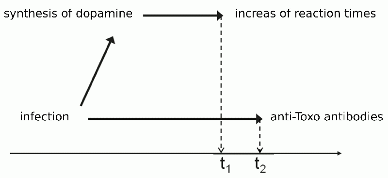
Fig. 11 An example of the failure of the temporality criterion. In a test, we may find that some people have longer reaction times before we detect (using the antibody test) that they have toxoplasmosis, even if/though the prolongation of reaction times is due to toxoplasmosis. This is a hypothetical and actually not too probable an example. It is more likely (but not certain) that specific antibodies appear before the infected person attains a longer reaction time.
Figuring out whether toxoplasmosis induces changes in the psyche, or whether psychological differences affect the risk of infection – in other words, determining cause and effect – wasn’t an easy nut to crack. But again, we got lucky. In our department, we closely cooperated with the diagnostic laboratory of the Prague Hygiene station. The researchers of this lab kept long-term records of people who had been tested for toxoplasmosis. And these records contain not only the result of the toxoplasmosis tests, but also the addresses of the tested individuals. Back then, the Czech Republic didn’t yet have laws about handling personal data, so we could afford to do something we probably couldn’t (or at least shouldn’t) do today. We looked up the addresses of the patients, and wrote them a letter under the name of the diagnostic laboratory requesting their cooperation in a research project regarding the relationship between toxoplasmosis and human behavior. I didn’t tell them my suspicions that Toxoplasma changes human behavior, because I expected this might terrify a number of normal people. So most of the patients probably thought that we’re studying how behavior impacts one’s risk of infection. That was partly true, since we also included a couple of questions regarding risk factors, such as consumption of raw meat and unwashed vegetables, contact with soil, and the size of one’s residence. In contrast, the University scientists and biology students (I was going to write “abnormal people,” but finally changed my mind – there’s no need to insult the reader’s intelligence with overexplicitness) who served as subjects in the first study were usually excited at the possibility that a parasite manipulates human behavior, and therefore were happy to be guinea pigs in my study. Approximately 80% of the biologists I asked agreed to participate – even today, this seems quite incredible to me.
But back to the former patients we looked up in the records of the diagnostic laboratory. In cooperation with the researchers of this lab, we sent out about 500 letters. This first wave of letters went to men who had been tested for acute toxoplasmosis within the last twelve years and came out Toxo positive. I hypothesized that if Toxoplasma truly changes human behavior, then the psychological changes should become more profound over time: Superego Strength (G), and maybe Self sentiment integration (Q3) and Affectothymia (A) should be lower in long-infected men, and Suspiciousness (Protension, L) greater, than in recently-infected men. We sent the questionnaire only the men whose time of infection we knew. Fortunately, this can be determined according to levels of group IgM antibodies in the blood; these antibodies increase in infected persons, and usually peter out within half a year (see also Box 22 Antibodies and myths about them). We got back a good number of completed questionnaires, so in the end we had data on the psyche and time of infection of 190 men. The question we wanted to answer with this data was simple: Do the factors of suspiciousness and superego strength change with time after infection in the expected direction, that is, with suspiciousness increasing and superego strength decreasing (Box 17 Checking and cleaning data)?
Box 17 Checking and cleaning dataThere is no data set so small that it does not hide at least one erroneous item. Perhaps there is or was an exception somewhere (probably at the edge of the world), but I haven’t found it yet. When you finish collecting data and are getting ready to analyze it, you must suppress the curiosity to look at the results. Before seeing your results, it is imperative that you carefully check the correctness of the data. Otherwise you risk becoming enamored with the data, and become reluctant to check them – in which case, any observed association may be due to errors in the data. Besides, part of data checking is revealing and dealing with outlying values. And you have to decide what defines an outlier, and whether you should leave it out or perhaps replace it with the average value, before approaching any sort of analysis. If you do it after the analysis, you risk eliminating “unfitting” extreme values and keeping only values which support your hypothesis. You must check the data for values that are too high or too low; negative values where data can only be positive (body mass, age); for text mixed in with digits (if you mix up the zero and O on the keyboard, a “number” like 1OO can cause you many a headache later on). There’s probably no ideal way to check data. But you can’t go wrong if you create a histogram of the distribution of each studied variable; and perhaps even an XY-graph of the relationship of each pair of quantitative variables. When looking at the histograms, you can not only find dubious data but also immediately recognize that some variables should be transformed before the analysis (for example, by taking their log), in order to obtain a symmetrical, and if possible, normal distribution (see Box 18 Data transformation). |
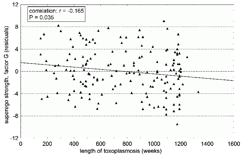
Fig. 13 The factor Super Ego Strength (Cattell’s factor G, Rule-consciousness) decreasing with time after infection by Toxoplasma. The test subjects are male patients who were diagnosed with acute toxoplasmosis in the past. The date of acute toxoplasmosis was estimated on the basis of clinical symptoms and the transient increase in the levels of IgM antibodies against Toxoplasma. One hundred sixty four patients participated in the study. Because one’s psychological profile can change with age, we statistically filtered out the age of the subjects. The graph represents standardized residuals after this analysis.
Analysis of the data showed that two Cattell’s factors, specifically superego strength (Rule-consciousness G) and Self sentiment integration (Q3), decrease with time after infection (14) (Fig. 13). So we concluded that Toxoplasma changes a person’s behavior, as opposed to a particular behavior increasing the likelihood of Toxoplasma infection. At the very least, this applied to the factors of Superego Strength and Self sentiment integration; in this study, we did not prove a correlation between suspiciousness and time after infection. And I must admit that to this day I’m uncertain if there is a relationship between toxoplasmosis and suspiciousness. Whereas superego strength is almost always different in infected versus uninfected men, differences in suspiciousness can only be seen in a couple subject groups.
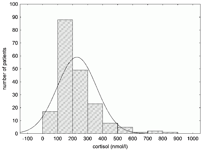
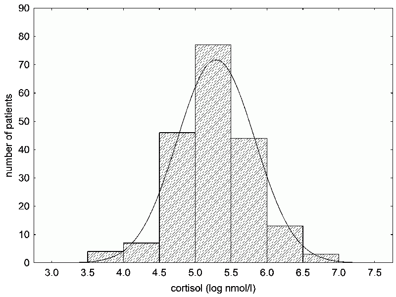
Fig. 12 An example of data (the concentration of the stress hormone cortisol in the serum immunology clinic patients) that do not have a normal distribution (a), but which can achieve one through logarithmization (b). Data sets without normal distribution, particularly small ones, cannot be analyzed with common parametric statistical tests, for these tests may produce incorrect (usually false positive) results. Therefore, it is necessary to use nonparametric, randomized or exact tests. For large data sets, a non-normal distribution usually isn’t an issue – in this case, applying parametric tests to our data did not produce biased results. Distribution type can be determined using the appropriate statistical tests. However, in small data sets, for which knowing the distribution type is especially important, deviations from normal distribution are often valued as not significant. In contrast, these deviations are almost always significant in really large sets of data. Therefore, it’s better to always check the shape of the distribution visually.
Box 18 Data transformationMost common statistical methods expect and more or less require a normal (Gaussian) distribution of values in the data set. A normal distribution has few high and low values; most of them cluster around the average. A histogram of a normal distribution is a characteristic bell-shape. Many values we measure in nature, such as body height, usually have such a distribution – or, more accurately, they do not differ much from it – but others do not. A common example is the log-normal distribution, an asymmetrical bell-shape whose right side (the side with the higher values) decreases at a much lower rate than the left side. A log-normal distribution can be transformed into a normal one by taking the logarithm of the measured values. If the measured values include zero, then we must add a small constant to all the values before taking their log, because the log of zero is undefined (Fig. 12). Sometimes, the histogram remains asymmetrical even after it been logarithmized – in which case we can logarithmize the values a second (and maybe even a third) time. In general, you can make as many transformations of the data as you need. The results won’t be distorted; rather, the statistical test becomes more reliable, the closer the data resembles a normal distribution. Only, when describing your results in the manuscript, you must keep in mind that differences in the logarithms of the heights – not the differences in height (of, for example, infected versus uninfected people) are statistically significant. There isn’t really a substantial difference, but the reviewer of your article might give you trouble over it. Even if you’re using statistical tests to compare things like the logarithms (or perhaps arc sines) of heights, plot the axis with height in non-logarithmic units (such as centimeters). In this case, the graph should first and foremost be illustrative and clarifying, and height expressed in centimeters better suits this purpose than height in logarithmic values. |
While waiting for letters from the former patients, I continued collecting data in the College. I had already “picked through” most of the employees, so I now focused my efforts on the students – particularly the female students. The fact that I had originally not found statistically significant differences between infected and uninfected female students may have been because toxoplasmosis really doesn’t affect them; or it could have been because there were too few women in the original subject group. After a year or two, our College subject group numbered 224 men and 170 women. When it was finally analyzed, it turned out that women with toxoplasmosis are likely to have psychological differences, which are primarily in the factor A, Affectothymia (Warmth). Affectothymia is actually the factor which most influences a human’s personality profile. It accounts for the majority of differences among people in their psychological characteristics, coming just before intelligence. Women infected with Toxoplasma had a statistically significantly higher factor A than did uninfected women; therefore, they were more sociable and open, but also more flighty. In contrast, uninfected women were rather closed-up and less sociable, but also more conscientious and responsible. Aside from this factor, there was a clear shift in Rule-consciousness (Superego Strength, G) and suspiciousness (Protension, L), which were the same factors that had been different in Toxo positive men. But what was interesting, was that these factors were shifted in the opposite way in women than in men – uninfected women had greater Superego Strength, meaning that they were more willing to respect social norms and were less suspicious. This trend (the opposite relationship in men than in women) was seen in a number of other factors, including the factor Affectothymia, which in later subject groups was often lower in infected men. But most of the time, this was only a trend that did not prove to be statistically significant in women or men.
While collecting the new data, I managed to publish our first findings in an international journal. It wasn’t easy; many journals sent the manuscript back. It wasn’t that the reviewers had found any glaring errors – but to most of them, the idea that some parasite might affect the behavior and psyche of a human seemed bizarre enough, that they preferred to think we invented our data (Box 19 Why not to mess with data and fabricate results). Finally, the first article was published in the Czech, albeit printed-in-English journal Folia Parasitologica (15); three years later, the second article came out in the British journal Parasitology (14). The second article also contained the results from the former patients with acute toxoplasmosis.
Box 19 Why not to mess with data and fabricate resultsAudits conducted by American officials on random samples of articles, showed that about 7% of studies published after 1985 include fundamental violations of scientific ethics (falsified data or plagiarism). Before 1985, it was 12%. Surveys of researchers show that many of them at some point falsified their data. Usually this means that they bettered their results – for example, by omitting unfitting values or failing to mention the unfavorable results of certain analyses. An even greater percent of scientists – that is, 32% – believe that their colleagues sometimes “tweak” their results. So we should approach other people’s data with a certain wariness. We cannot rule out even the unlikely possibility, that all of the data is made-up, or fundamentally modified. So why not falsify our own results, instead of dealing with rebellious data that may be difficult and costly to obtain, and which oftentimes ruins our brilliant hypotheses? I won’t delve into the ethical reasons; for example, that lying and cheating is wrong, and that people generally enter into science because they want to figure out how our world works – and clearly, falsifying data is the basest way to betray this calling. I realize that ethical reasons depend on the individual, and are not universally agreed upon; and so, for example, a PhD student or technician in a Japanese laboratory might see it as ethically more correct to please one’s sensei and laboratory head by falsifying the results to obtain favorable data, rather than disappoint him with true results that refute his theory. No, the obvious reason we shouldn’t falsify data is something else. If we published important and interesting results that were actually falsified, then other scientists would soon find out when trying to repeat our study. And falsifying unimportant and uninteresting data also doesn’t pay off: is easier and, from a career stand-point, more secure to collect unimportant and uninteresting data – there is tons of it available. (There’s also tons of interesting data around us, but to find it, you must know how to look.) |
In the first article, I managed to cram in an observation that I can’t puzzle out even today. When looking at infected versus uninfected College employees, I saw one big difference. Among fourteen men with toxoplasmosis, there was only one who had some sort of leadership position, such as the department head or dean. But out of 29 Toxo negative men, there were ten people with leadership positions. In truth, this corresponded with the results we obtained from the questionnaire. If someone isn’t willing to follow social norms (has a lower factor G), then getting a leadership position in an institution like the University cannot be easy. That one outlying Toxo positive man was the department head for only two years, and had risen to the position by way of the revolution. Back then, department heads were still chosen based on personal and professional qualities, rather than progression through the social hierarchy and consolidating a position of power. I don’t know if this dependency still applies. Many Toxo positive professors later became department heads. But even so, I expect that if we compared how many years Toxo positive versus Toxo negative men spent as department heads, then the difference would be perhaps even greater today than in the past.
I knew that Toxoplasma apparently affected not only male behavior, as seen in the first study, but also female behavior, as shown in the second study on the students of the College of natural sciences. So I decided to supplement the first study with data from the former patients with acute toxoplasmosis – using data from the female patients. With the help of the workers of the diagnostic laboratory, I was able to amass psychological data from 230 female patients, who had had acute toxoplasmosis within the past 14 years. For this subject group, we plotted the factors of Affectothymia (A) and Superego Strength (G) against how long the person had been infected. It turned out that the correlation with factor G is statistically significant – Superego Strength increases with time after infection (see Fig. 14). On the other hand, Affectothymia – the factor which correlated most with Toxo positivity in
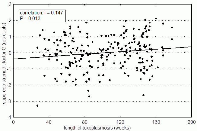 |
Fig. 14 The factor Super Ego Strength (Cattell’s factor G, Rule-consciousness) increasing with time after infection by Toxoplasma. Subjects are female patients diagnosed with acute toxoplasmosis in the past. The date of acute toxoplasmosis was estimated on the basis of levels of IgM antibodies against Toxoplasma. Two hundred thirty patients participated in the study. Because one’s psychological profile can change with age, we statistically filtered out the age of the subjects. The graph represents standardized residuals after this filtration.
female students – did not change with time after infection. Of course, just like in the previous study with male patients, I filtered out the effect of the person’s age. It could be expected that women who’d been infected longer were, on average, older at the time of the study; and therefore psychological factors which normally change with age could have been higher or lower in longer and shorter-infected people. But with modern statistical methods, it’s not difficult to filter out such confounding factors (see Box 20 Dependent, independent, and confounding variables; fixed and random factors). Besides Superego Strength, several other factors changed with time after infection. At this point, I’m not sure why there was no change in suspiciousness and Affectothymia in women. I may have just been unlucky with this data group. Statistical tests allow us to estimate the risk of a type I error, in other words the statistical test tells us that the difference in Warmth between infected and
Box 20 Dependent, independent, and confounding variables; fixed and random factorsWhen conducting statistical analysis, we must first determine what is the independent and what is the dependent variable, because this usually determines not only how we interpret the results, but also the statistical method we select. An independent variable, also known as a factor, is a variable whose effect we wish to study. On the other hand, a dependent variable is a variable which is affected by the independent variable. So if we’re studying how toxoplasmosis affects the suspiciousness of students, then toxoplasmosis is the independent and suspiciousness (based on Cattell’s factor L) the dependent variable. Of course, there can be several independent variables which affect our independent variable, including toxoplasmosis, gender, profession, age (age is a continuous variable, and independent continuous variables are also known as covariates). But let’s say we’re studying what all affects the risk of Toxoplasma infection. In this case, Toxo positivity is the dependent variable and things like age, gender, consumption of raw meat, contact with cats, and nationality are independent variables. It’s useful when we can include all our independent variables in the statistical test at once, because, among other things, it allows us to reveal any possible interactions – for example, toxoplasmosis may affect suspiciousness differently based on gender. Sometimes we’re not actually interested in the effect of a particular independent variable, but we know that it affects our target variable, so therefore we must filter out its effect in order to reveal the (perhaps weaker) effect of the variable we are studying. To this end, we include it among the other independent variables. Such a variable is called a confounding variable. It’s also important to know whether an independent variable is a fixed or a random factor. A fixed factor (such as gender) has a set number of possible values objectively determined, for example, by nature; whereas a random factor (such as profession or nationality) has a random number of possible values subjectively chosen by the researcher. A statistical program deals differently with these two types of variables.
|
probability that the phenomenon we see in our data doesn’t actually exist – that it’s just the result of chance. Let’s say the uninfected women is significant at the 2% level. So there is a 2% chance of obtaining this or a more extreme difference between two groups due to chance – in other words, because a different number of Warm women happened to get into the Toxo positive versus the Toxo negative group. Of course, a statistical test can never give us complete certainty, but if we obtain a sufficiently low P value (significance level), then we can lean towards the conclusion that the observed phenomenon is real – for example, that there exists some relationship between Affectothymia and toxoplasmosis. Generally, we can lean towards this conclusion if we get a P value lower than 5%, but this level is arbitrary, so its importance should not be overestimated. If you have observed an interesting phenomenon, such the effectiveness of a new drug in treating cancer, then it’s worthwhile to pursue it even if you get a P value of 10% – in other words, that the drug doesn’t actually have an effect, and that people who got the drug are just as well (or poorly) as people who got the placebo. On the other hand, we’ll probably abandon a more trivial phenomenon, such as that the new drug lowers the frequency of blinking, even we get a P value of less than 5% (assuming, of course, that we aren’t being paid by a Formula One stable to find an anti-blinking drug). Similarly, if verifying the existence of a phenomenon is fast, easy, and cheap, then we’re more likely to pursue even a phenomenon with high P values; whereas if such verification through an independent study is difficult or expensive, then we’re likely to pursue it only if the P value is extremely low – maybe 0.1%.
Besides the type I error, there also exists a type II error, which occurs when a statistical test refutes the existence of a phenomenon that actually exists. The probability of a type II error is determined by the strength of the test. The greater the strength of the test, the greater is the probability that the test will reveal the real phenomenon’s existence. For mostly historical reasons, scientists are more afraid of type I than type II errors (maybe they would rather miss an existing phenomenon – nobody will ever know about their failure - than suffer the embarrassment of proving the existence of a non-existent phenomenon). The probabilities of type I and II errors are somewhat related, and statistical tests are set up so that when we require a type I error of less than 5%, then we’ll get a high type II error, maybe around 20%. This means that in one out five studies, on average, the statistical test will refute the existence of a phenomenon that truly exists (see Box 21 Analysis the power of a statistical test).
Box 21 Analysis the power of a statistical testIf we’re not interested in the probability of a type I error (the risk that the observed phenomenon is just the result of chance), but rather in the likeliness of a type II error (the risk that we incorrectly identify a real phenomenon as nonexistent, purely the result of a chance), then we must use the correct method of power analysis. This technique is primarily used for two things. The first is determining the extent to which we should trust the negative results of a study, which don’t prove the existence of the phenomenon we expect. The second is related to the planning of the study. Power analysis allows us to estimate the size of an experimental group – i.e., the number of human subjects or lab mice – needed for us to have a good chance of proving an effect of a certain size (Fig. 15). Various statistical tests differ in their strength, which means that they carry different risks of a type II error. For example, nonparametric tests usually have a lower strength than parametric ones; so whenever the data type allows it, we should preferably use a parametric test – or perhaps an exact test, which is even stronger. |
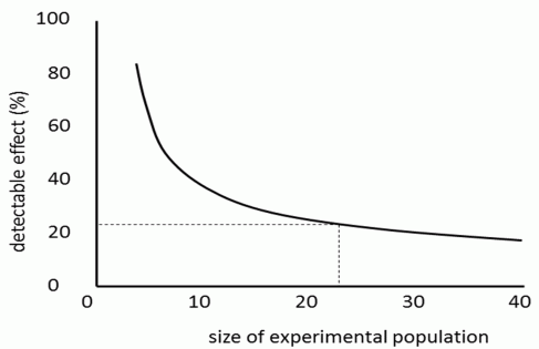
Fig. 15 Power analysis. The result of a power analysis can look like this graph. If we had an effect that caused a 20% difference – for example, if Toxoplasma decreased the weight of infected mice by 20% - then 22 experimental mice would probably be enough to prove it. But if Toxoplasma decreased weight by only 15%, we would probably fail to prove the effect to be statistically significant, even if we had 40 mice
And this might’ve been what happened in the afore-mentioned study with the female acute toxoplasmosis patients. We expected that Affectothymia (warmth, openness and sociability) would increase with time after infection, but the statistical tests did not confirm it. So why do I suspect it was the fault of a type II error, i.e. a mistaken refutation of an existing phenomenon? Because immediately afterward we carried out another study with a somewhat different method and a completely different group of people, and this study did prove an increase in warmth and sociability with time after infection. One of my colleagues had, filed away in his desk drawer, data from a large group of women who had been screened for toxoplasmosis during pregnancy. We had no psychological data for these women, but on the other hand, the data set was very large – almost a thousand women. Next to each name was the woman’s address, screening result, weight, and then two mysterious values marked Pm and Uz. I later found out that Uz was the duration of pregnancy based on an ultrasound – in other words, based on the size of the fetus – and Pm was the duration of pregnancy estimated from the date of the last menstruation. Both of these durations related to the time of the screening. Again, they were at first only mysterious values to me. I didn’t expect that they might be related to toxoplasmosis. I entered all the data into the computer, including these three values: the weight, the duration of pregnancy according to ultrasound, and the duration of pregnancy according to menstruation. These three values proved to be quite interesting; their analysis led us to an entirely new area of studying Toxoplasma’s effect on the human organism – but that’s a matter for a different chapter. We sent our ten questions mixed into Cattell’s questionnaire to all the Toxo positive women, as well as to a random sample of Toxo negatives, and requested their cooperation in the name of the National Institute of Public Health.
This time fewer people responded and we obtained completed questionnaires from only 20-30% of the women. Partly, it was because the women now had children, and probably had little time for the questionnaire; and partly, it was because we intentionally refrained from discussing the goals of the study in the accompanying letter, to avoid needlessly frightening the women with the mention of a parasitic protozoan, Toxoplasma. I compared the psychological factors in infected and uninfected women; and using the subset of infected women, I tried to determine whether the psychological differences increased with time after infection. But of course, I didn’t know how long ago these women had been infected. I could’ve at least estimated it based on the levels of their Toxoplasma antibodies. This parameter is highly variable over time, and depends on the state of a person’s immune system, so antibody levels cannot determine how long ago someone was infected (see also Box 22 Antibodies and myths about them). Some people have high antibody levels, and others have low ones. Furthermore, antibody levels in an individual change over time. Nevertheless, on average, they decrease with time after infection. So if we have two women with different antibody levels, we cannot definitely say which one was infected earlier. But if we have ten women infected five years ago, and ten infected two years ago, then it’s almost certain that the average level of antibodies will be lower in the first than in the second group of women. So, statistically, there exists a relation between antibody levels and time after infection. And if we’re looking for a statistical relationship, such as a relation between a psychological factor and time after infection, then we can look at the factor in relation to antibody levels, in place of time after infection. We can, on average, expect that the longer the time after infection, the lower the levels of antibodies; and the lower the levels of antibodies, then the greater the difference in the psychological factor. And the results of our study did show that antibody levels correlate with both factor A and G. In both cases, the factor changed in the direction that we hypothesize based on our theory and data we had obtained from students at the College. The factors of Affectothymia (warmth, A), and Superego Strength (rule–consciousness, G) increased with decreasing antibody levels. Several other factors also changed with decreasing antibody levels: for example, Protension (suspiciousness, L) decreased, Surgency (enthusiasm, heedlessness, F) increased, and Social Boldness (H) increased. So we once more confirmed that changes in women’s psyche occur after Toxoplasma infection, and therefore are induced by it (16).
Box 22 Antibodies and the myths about themAntibodies are proteins whose biological role is to lock onto to foreign structures. These foreign structures, called antigens, often come from parasites. After an antibody binds to them, they are eliminated either directly by the antibodies or by specialized cells like macrophages, which detect and devour antibody-marked antigens. The antibodies are created in B cells, which are a type of white blood cell. Each B cell creates only one type of antibody to target one antigen (or more accurately, to target a small area on the antigen, known as the epitope). The body contains many B cells, and therefore can produce millions of different antibodies, capable of binding to millions of foreign structures with the individual has not yet encountered – including molecules created in the laboratory by man, and which weren’t present in nature before. A healthy individual, or rather someone who doesn’t have an autoimmune disease, doesn’t make antibodies that would bind to structures found in his own body. The presence of antibodies against a certain microbe, usually a parasite, in the blood is commonly used to diagnose infection, since it’s often much easier to detect antibodies than the actual parasite. According to the type and concentration of the antibody, it’s often possible to determine the phase of infection. Soon after infection by a pathogen, class IgM antibodies appear in the blood. These decrease over time, and instead class IgG antibodies reach their peak. Once the acute stage passes, the amount of antibodies gradually decreases (but often they start binding more strongly to the antigens). If the antigen disappears from the body, then the antibodies disappear eventually, too. But a small number of the B cells that produced the antibody remain in the body as memory B cells, which create a person’s immune memory. So in the future, if the body encounters the same antigen (for example, the same parasite), then the memory B cells can quickly divide and begin producing the respective antibody – in this case, they immediately release class IgG antibodies, which are capable of strongly binding to the antigen. This is called a secondary immune response. The parasite is eliminated by the antibodies and various white blood cells soon after penetrating the host body, and the acute disease is either much weaker or never happens. A number of myths about the formation and function of antibodies are senselessly reprinted from textbook to textbook, even though modern immunology has long refuted them. For example, it’s not true that antibodies serve to differentiate between foreign and self antigens. In reality, this function is performed by T cells, which do so based on the presence of unknown peptides (short amino-acid chains) from the proteins of a parasite, or from the antibodies that bind to the antigen. Antibodies serve to mark foreign structures, but the structures must first be distinguished as foreign by the T cells. It’s also not true that the body has B cells capable of producing antibodies against all possible antigens ahead of time; and these B cells only need to start reproducing when an antigen enters the body. In reality, the B cell clones which produce antibodies that firmly bind to the foreign antigen but don’t bind to self antigens, are “bred” by T cells in specialized immune organs only after the foreign antigen has entered the body. T cells do this in a similar fashion as a person breeding new variants of crops or farm animals. On their surface, B cells have molecules of the antibody they produce. These molecules constantly bind (sometimes not very strongly) to structures from both parasites and the self. These structures are then absorbed by the B cell, and if they contain proteins, then these get digested into small peptides. The peptides bind to strange transport molecules, known as MHC-proteins (MHC-antigens), which transport them to the surface of the B cell and display (present) them (see also Box 36 On peptides, and why they should interest a parasitologist). The B cells are constantly surveyed by T cells, which “feel” for the peptides presented on the MHC-antigens. Each T cell recognizes a certain peptide, but these are only peptides not present in the body’s own proteins. This is because young T cells which detect peptides present in the body are killed when passing through the thymus (this is where T-cells get their name). So as soon as a T cell recognizes a peptide presented by a B cell’s MHC-proteins, it’s clear that it must be a foreign peptide (it was not present in the thymus). And the B cell which just proved itself capable of binding to an antigen (a structure containing at least some foreign peptides), is given a dose of growth factor from the T-cell, allowing it to reproduce. The “clones” of the B cell should produce the same kind of antibody as the original B cell. But the gene coding for the antibody is subject to frequent mutation, so the offspring produces variations of the original antibody. Some bind to the antigen more or less strongly, some also bind to self-antigens, whereas others lose the un-wanted ability to attach to them. Of course, the mutated B cells whose antibodies bind best to the foreign antigen and not to self-antigens (which would fill up their surface receptors, and thus limit their ability to bind to foreign antigen) are the most likely to bind to the antigen. So these B cells are most likely to absorb the antigen, present more respective peptides, and hence get more shots of growth factor from the T cells. The B cells again reproduce and obtain new mutations, some of which improve their ability to bind to the given antigen (or lower their ability to bind to self-antigens). And the B cells with these “good” mutations are again made to reproduce the fastest. Over several days and a couple of generations, the T cells will have bred a B cell clone which produces antibodies that bind very firmly to the foreign but not to self-antigens. |
Later we confirmed our conclusions on results obtained using the more modern Big Five questionnaire. It turned out that the factor Conscientiousness (which is lower in Toxo positive humans, as mentioned in the previous chapter) decreases in infected men and women with time after infection. However, the decrease was statistically significant (and very significant, at that) only in men.