XIX. Why infected women have longer pregnancies – the effect of toxoplasmosis on fetal development
I’m repeating myself already, but I must start by saying that chance often played a large role in our studies. On one such occasion, chance was responsible for our discovering that latent toxoplasmosis affects the course of pregnancy. As I already mentioned, one of our subjects groups on which we were studying the effect of toxoplasmosis on the human psyche, included data regarding pregnant women who were screened for toxoplasmosis around their 16th week of pregnancy. Each woman had been determined to be 16 weeks pregnant according to two methods: the results of the ultrasound from her first visit to the obstetrician, and according to the starting date of her last menstrual cycle. Therefore, we had four pieces of data for each woman: the result of toxoplasmosis testing, the length of pregnancy determined by that ultrasound examination, the length of pregnancy according to the date of her last menstruation, and her weight at the time of the toxoplasmosis screening. Unfortunately, we had no data on her body weight at the beginning of pregnancy. For curiosity’s sake, when entering these four pieces of data into the computer, we tested to see if Toxo positivity correlated with any of the other data. Statistical testing quickly revealed that Toxo positive women had a greater body weight at the time of the toxoplasmosis screening. Also, when using the menstrual cycle (but not the ultrasound) method to estimate the duration of pregnancy, Toxo positive women appeared to have been pregnant longer than Toxo negative women.
First we’ll look at pregnancy weight, because it’s a simpler relationship, but still very interesting in terms of both the research methodology and health implications. Toxo positive women in their 16th week of pregnancy had a greater body weight than did Toxo negative women. But when we plotted a graph of Toxoplasma antibody levels versus body weight, we observed something strange there was a positive rather than negative correlation between the antibody levels and body weight. The lower the antibody levels of a woman –the longer she’d been infected with toxoplasmosis – the less she weighed in her 16th week of pregnancy. For a long time, we couldn’t to reconcile these two contradicting results. Finally, it occurred to us that it could be because of the women who were infected for the longest time – the women who had such low antibody levels that we falsely diagnosed them as Toxo negative. Because of this false classification of the longest-infected – and therefore also the lightest women – among Toxo negatives, we may have gotten the average weight of infected women seemingly lower than that of uninfected women.
This hypothesis, which supposes a false diagnosis in a significant portion of Toxo positive women, was, “surprisingly” enough, not appreciated by our colleagues who were carrying out the toxoplasmosis screening. It was also clear that it would be difficult to test this hypothesis, if only because we no longer had the original samples available, and so we couldn’t repeat the serological tests. Finally, we tackled the problem using a test specially developed for this issue. It was not a statistical test, but a permutation test. Permutation tests belong among randomization tests, which can be used for a similar purpose as statistical test. In comparison to statistical tests, randomization tests have a number of advantages, and among other things, they can be much more easily adapted to a specific case. A permutation test is conducted by first electing a parameter that would reach a higher (or lower) value if a particular factor had an effect (such as the effect of toxoplasmosis), than if this factor had no effect on the data. For example, if we’re interested in knowing whether Toxoplasma affects the weight of mice, we select as our parameter the difference between the average weight of infected and uninfected mice groups, and estimate the value of this parameter from our experimental data. Then we permute the experimental data – we randomly change the order of the weight values of all the mice in our file, regardless of whether the mice were infected or uninfected. And again we calculate our parameter for the re-ordered (permuted) data. After permuting the data many times, such as 999 times (of course, the computer does it for us), we finally have available 1000 values of the parameter, one of which was calculated for the real data and 999 calculated for re-ordered data. We order these values from smallest to largest and see where our not jumbled up data value winds up. If it’s among the 2.5% lowest or 2.5% highest of the values, we can conclude that the given factor (toxoplasmosis), probably affects the weight of mice (Box 82 One- and two-sided tests).
In our case, we developed a permutation test which allowed us to filter out the effect of the incorrectly diagnosed Toxo positive people – that is, the women who had such low antibody levels, that they were falsely classified among the Toxo negatives (90). We conducted the test by taking our data from about 760 pregnant women, which included their body weight throughout pregnancy. A previously selected percent of the Toxo negative women with the lowest weight was moved by our computer into the group of Toxo positive women – in four independent tests we tried reclassifying 5, 10, 15 and 20% of these Toxo negative women. After moving the lightest Toxo negatives into the Toxo positive group, the computer program calculated the average body weight of each group, and then found and stored in its memory the difference of the two averages. Then it randomly jumbled up our data (permuted it). Without regards to Toxo positivity, it separated the women into two groups which corresponded in size to the original Toxo positive and Toxo negative groups. Then the computer again moved the given percent of the lightest women from the subgroup that corresponded size-wise to the original Toxo positive group, into the group that corresponded to the original Toxo negative group. For both permuted subgroups, the program calculated the averages, and finally calculated and memorized the difference between these averages. The entire procedure of forming permuted groups was subsequently
Box 82 One- and two-sided testsIf we test the hypothesis, that a certain factor (maybe toxoplasmosis) somehow affects (we don’t know how beforehand) a certain trait of an organism (such as intelligence of the test subjects), we must use a so-called two-sided test. Using this test we estimate the probability that the given factor does not affect the studied trait – we compare this probability with the probability the factor does increase or decrease this trait. In some cases we expect ahead of time that the given factor affects the studied trait in a specific manner, perhaps by lowering it. In the first study we may find that toxoplasmosis increases the intelligence of infected women, and in another experiment we try to verify this finding on independent data. Or we discover that toxoplasmosis increases body weight of infected people, and then subject this data to two independent tests to determine whether the given effect occurs in both men and women. In such a case we use a one-sided test, which allows us to estimate the probability that the given factor doesn’t influence or lowers the studied trait – we compare this probability with the likelihood that the factor increases the studied trait. Some statistical programs automatically give you the results of both the two-sided and one-sided test; other times we must calculate on our own the results of the one-sided test from the results of the two-sided test, usually (but not olways) it’s very simple – we divide the value P from the two-sided test by two. Before the age of computers, the significance of a test was determined using statistical tables. In these tables, one found whether the calculated value of the test, in our case the t value, represented a statistical significance at the 5% (or 1% or 10%) level for a given degree of freedom, i.e. whether the probability of obtainin our data or more extreme data due to chance is lower than 5% (or 1% or 10%). When calculating a one-sided test, a researcher used the same tables as for a two-sided test, but considered results of the test to have 5% statistical significance when he found 10% significance in the tables. Of course, we must have a good reason to use a one-sided test (and a good reason most certainly isn’t that we failed to find statistical significance using the two-sided test), and we have to decide to use it before starting data analysis. |
repeated many times, in our case 2999 times, so finally we were left with 3000 values, the difference in average body weight of the groups of women. And one of these 3000 values was the difference calculated from the original data, and the other 2999 values were the differences calculated from randomly jumbled up data. The last step was to look in what percent of the highest or lowest values the real-data value was found.
The results of the permutation test were unambiguous. We only have to move 5% of the lightest Toxo negative women into the Toxo positive group for our permutation test to show that Toxo positive women have significantly lower weight (as opposed to significantly greater, as we saw using the original data set). The value which expressed the difference between the average body weight of Toxo positive and Toxo negative women was found among the 2.1% lowest values. From this one can conclude that the observed difference in body weight between Toxo positive and Toxo negative pregnant women probably wasn’t due to chance. The paradoxical finding that Toxo positive women have a greater body weight than Toxo negative women, even though women infected longer weigh less than those infected more recently, was most likely caused by incorrect identification of certain Toxo positives. The women who were longest infected with Toxoplasma, and had the lowest weight, were placed as Toxo negatives due to the insufficient sensitivity of the serological test. And I was pleased that my cherished randomization tests once more triumphed over statistical tests (Box 83 Randomization tests).
Another curiosity we observed in our data was that the duration of pregnancy estimated according to the last menstruation, but not the duration of pregnancy estimated by ultrasound, was longer in Toxo positive than in Toxo negative women. That seemed to us both very interesting and very difficult to explain. From the start, we came up with several working hypotheses. One assumed that Toxo positive women conceived in a later phase of the fertile period of their menstrual cycle than did Toxo negatives. But the reason why this would
Box 83 Randomization testsThe probability of the hypothesis, that a certain phenomenon (for example, an average longer reaction time observed in Toxo positive people) is the result of chance (i.e. the probability of a so-called null hypothesis), can be estimated using three possible methods. Most often we use a statistical test, in this case most likely Student’s t test. Statistical tests give us only an approximate result, because regardless of the true distribution of the data in the subject group, the tests assume some standard shape of this distribution (usually a normal distribution). Statistical tests can also be nonparametric, in which case they require less assumptions about the parameters, e.g. the distribution of the data set, but nonparametric tests are usually weaker than the parametric tests, i.e. they have higher probability of providing false negativative results. This difference, however, is not very large and I usually prefere to use nonparametric type of the test whenever available. The precise probability of obtaining our or more extreme data under conditions of validity of the null hypothesis can be obtained using an exact test. Such a test uses combinatorial formulas to calculate how many different combinations can be made based on our data, and in what fraction of these combinations the studied effect is just as (or more) extreme as observed in our original data. For example, our program first calculates (or a stupidly written program uses the brute-force method of generating and checking all combinations) how many different ways the 760 pregnant women can be divided into two groups of sizes that correspond to the size of the Toxo positive and negative groups. Then it calculates what percent of these combinations has an equally larger or larger difference in average body weight between the two groups, as was found in the original data. The third way to determine the probability of obtaining our or more extreme data under condition of validity of a null hypothesis and therefore to estimate the validity of null hypothesis is to use a randomization test. Randomization tests are similar to exact tests, but instead of finding the fraction of all possible combinations with equal or (more) extreme values than seen in the real data, we only find this fraction out of a randomly created sample (for example, out of 1000 random combinations). The accuracy of the test’s result depends on the size of the sample we use; from a practical standpoint, it depends above all on our patience and the speed of the computer. Randomization tests can be divided into permutation tests and Monte Carlo tests. Permutation tests compare real data with many samples of data created by permutations (random mixing up) of this real data. Monte Carlo tests compared real data with many samples of data generated using our model of the observed phenomenon. Let’s say that we want to use a Monte Carlo test to estimate the probability that playing dice are false. When we throw ten dice and find that nine of them land showing a 6, we let the computer “throw ten dice” ten thousand times, and calculated what percent of these “throws” gave nine or even ten 6s.
|
occur wasn’t apparent. We considered both physiological and ethological mechanisms – for example, a change in the frequency of sexual intercourse. If Toxo positive women had less frequent sexual intercourse, one might expect that on average they become pregnant later than Toxo negative women. But why would Toxo positive women, who test as more welcoming, sociable and frivolous, have less frequent sex? Let’s think along the lines of good ol’ gender stereotypes. Maybe the Turkish researchers who revealed that infected women suffer more often from migraines are right (75).
Another working hypothesis, more serious in its implications, was finally shown to be true. It states that Toxoplasma slows the development of the human fetus. If the duration of pregnancy is determined from an ultrasound taken at the time of the woman’s first visit to the obstetrician, then a fetus which develops more slowly will appear smaller and therefore younger, so the doctor will falsely estimate a shorter duration of pregnancy. Since a doctor usually screens women for toxoplasmosis in their 16th week of pregnancy based on the results of an ultrasound, rather than accordingly to less reliable data – such as the day the women remembers that she had her last period – he probably gives Toxo positive women a later appointment than to Toxo negative women. Therefore, the total duration of pregnancy if estimated from the date of the last menstrual cycle appears to be longer at the time of Toxoplasma screening.
We tried to test this hypothesis on other, unrelated subject groups (91). Collaborating with several gynecological laboratories from two private clinics, we gathered a wide range of data regarding the pregnancy duration of Toxo positive and negative mothers. Using this population sample, we confirmed that at the time of the regular screening conducted around the 16th week of pregnancy, the pregnancy duration of Toxo positive women was longer than that of Toxo negative women, when estimated using the date of the last menstruation, but not when estimated using the ultrasound examination. In this case, we also had available data about the total length of pregnancy, as well as the birth weight and length of the newborn. Thanks to this, we were able to prove that pregnancy in Toxo positive women on average lasts 1.5 days longer than in Toxo negative women (Fig. 44).
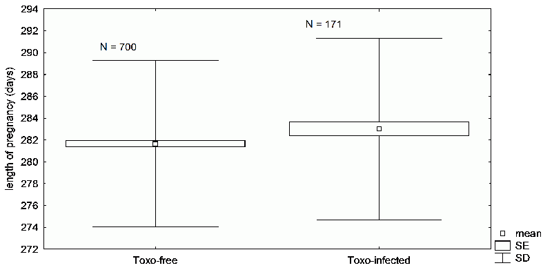
Fig. 44 The difference in the average pregnancy duration of women with latent toxoplasmosis and that of uninfected mothers. The difference is less than two days, but due to the low variability in pregnancy duration and the high number of test subjects, is considered statistically significant. You can very roughly estimate that the difference is statistically significant if the standard error rectangles don’t overlap.
That shows that Toxoplasma does slow the development of the fetus, probably in early pregnancy. Seeing as the newborns did not differ in birth weight or length, it’s apparent that the pregnancy lasts until the fetus reaches a sufficient size. Only then does the woman give birth. Originally, you see, we also had the hypothesis that infected and uninfected may have pregnancies of equal duration, but that the newborns of infected women were on average smaller.
It may seem that the 1.5 day difference in pregnancy duration due to toxoplasmosis is inconsequential when considering the general variability in pregnancy duration. In reality, the existence of even such a small difference could be important (Box 84 The size of an effect in a basic research).
The indication that that fetal development in Toxo positive mothers is slower than normal, and primarily in the earlier part of pregnancy, means that this effect might be accompanied by other defects. For this reason, in the next phase of our study, we observed the postnatal development of children born to Toxo positive versus Toxo negative mothers. Even here we found several interesting differences. It seems that children born to Toxo positive mothers also undergo slower postnatal development. When the children were about 2 year old, we sent the women we had screened for toxoplasmosis a questionnaire, which, among other things, determined the physical and mental development of the child. The women were asked when their child began lifting its head, when it started rolling over on its stomach, when it learned to sit on its own, when it began to crawl, when it began to walk on its own. In total, we got back completed questionnaires from 278 uninfected and 58 infected women. What was interesting, was that infected women who gave birth to a boy, were less likely to send us back a completed questionnaire than were the other women. After statistically filtering out the effect of the child’s birth weight (which we found did not correlate with the Toxo positivity of the mother), we saw that children of Toxo-infected mothers had statistically significant slowed development in all the areas we asked about, except for when they started walking. Since latent toxoplasmosis is not transmitted from the mother to the child, the children of Toxo positive women were not infected –
|
Box 84 The size of an effect in a basic research If, using a statistical test, we determine that a particular fertilizer raises the yield of a crop by 0.001%, it doesn’t make much sense to further study the possible applications of this finding. But unlike in applied research, in basic research the strength of the effect plays a much smaller role (see also Box 49 How to determine the effect size in statistics). In basic research, we’re interested in finding how the world around us works. We form individual hypotheses and progressively try to refute them using data obtained from simulations of the studied phenomena, or collected from experiments or observational studies. If our hypothesis states that a particular phenomenon does or does not occur under certain circumstances (for example, that the reaction time of infected persons worsens with time after infection), it is first important to determine whether this phenomenon exists – and not necessary to find how strong it is (for example, what percent of variability in people’s reaction times is due to time after infection). It doesn’t matter whether the length of infection explains 0.5 or 50% of variability in reaction time; either way, the results support our hypothesis that Toxoplasma worsens reaction time, and undermine the hypothesis that people with longer reaction times are more likely to get infected by the parasite. Of course, even scientists prefer strong effects to weak ones. Strong effects are less likely to be the indirect result of the influence of a different factor, a factor which we failed to include in our model. For example, a very weak correlation between time after infection and reaction time could be caused by the fact that some recently infected persons suspect that they had an infection (they recall suspicious symptoms), so they’re more interested in the study and try more in the reaction time tests. But there’s a similar (though somewhat smaller) risk also in the case of a strong effect. In science we must always approach results, our own and those of others, as provisionary, and we must also be prepared that they may mean something else than we originally believed (see Box 65 How hypotheses are tested in science?). |
nevertheless, their development was delayed. Of course, we can’t rule out the possibility that our results don’t show differences in the development of these children, but differences in how Toxo positive versus Toxo negative mothers perceive them. Or the results may be due to chance, and we may fail to replicate them on another test groups (Box 85 When and when not to use a Bonferroni correction).
Box 85 When and when not to use a Bonferroni correctionIt’s still a matter of contention, even among scientists, when it is and isn’t appropriate to conduct a Bonferroni correction for multiple tests in a basic research. To me it seems most reasonable to always apply a Bonferroni correction to multiple tests; but we cannot overestimate the results of the correction, whether it determines the tests to be statistically significant or insignificant. By applying sophisticated stepwise corrections, we can finally determine the probability that the observed result is due to chance. (We will be not able to determine it solely using a standard Bonferroni correction, i.e. by multiplying the obtained P values by the number of subtests; it would be necessary adjust not only the P values, but also number of tests in which the effect was statistically significant – using, for example, the stepwise Bonferroni correction or backward stepwise Bonferroni correction. But we usually need to determine, in which of the subtests the observed differences in the parameter are probably real and in which of the subtests they are probably due to chance. In such a case, a Bonferroni correction probably won’t help us – the only thing that’s left for us to do, is to repeat the study (preferably several times), to convince ourselves that the observed effect occurs in other, independent data.
|
We later found another very significant difference between Toxo positive and Toxo negative women. In one case, the observed effect was so strong that infected women reached on average a two times larger value in the studied parameter than did uninfected women. But these differences will be described in the next chapter.